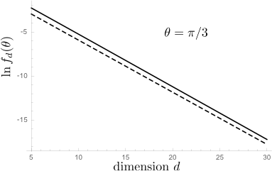
So I made this Gaussian approximation and find for $\theta=\pi/3$ a $d$-dependence of $f_d(\theta)$ that is well described by
$$f_d(\pi/3)\approx 2^{-d}e^{d/\pi^2}\Rightarrow g(\pi/3)\approx\tfrac{1}{2}e^{1/\pi^2}=0.553\;\;\;(1)$$
The plot shows the result of the Gaussian approximation (solid curve) and the asymptotic form (1) (dashed curve) on a log-normal scale, with a slope that matches quite well.
And here is the Gaussian approximation for several values of $\xi=\cos\theta$:
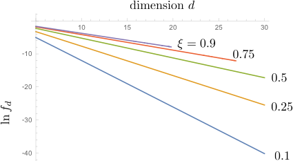
From the slope I estimate that
$$g(\theta)=\begin{cases}
0.66&\text{for}\;\cos\theta=0.9\\
0.63&\text{for}\;\cos\theta=0.75\\
0.55&\text{for}\;\cos\theta=0.5\\
0.41&\text{for}\;\cos\theta=0.25\\
0.25&\text{for}\;\cos\theta=0.1
\end{cases}
$$
Gaussian approximation
Denoting $\xi=\cos\theta$ we seek the probability
$$f_d(\xi)=2^d \frac{X_d(\xi)}{Y_d(\xi)},$$
as a ratio of the two expressions
\begin{align}
&X_d(\xi)=\int d\vec{x}\int d\vec{y}\, \exp(-\tfrac{d}{2}\Sigma_n x_n^2) \exp(-\tfrac{d}{2}\Sigma_n y_n^2)\delta\left(\xi-\Sigma_n x_n y_n\right)\prod_{n=1}^d \Theta(x_n)\Theta(y_n),\\
&Y_d(\xi)=\int d\vec{x}\int d\vec{y}\, \exp(-\tfrac{d}{2}\Sigma_n x_n^2) \exp(-\tfrac{d}{2}\Sigma_n y_n^2)\delta\left(\xi-\Sigma_n x_n y_n\right) .
\end{align}
(The function $\Theta(x)$ is the unit step function.) Fourier transformation with respect to $\xi$,
\begin{align}
\hat{X}_d(\gamma)&= \int_{-\infty}^\infty d\xi\, e^{i\xi\gamma}X(\xi)\nonumber\\
&=\left[\int_{0}^\infty dx\int_{0}^\infty dy\,\exp\left(-\tfrac{d}{2}x^2-\tfrac{d}{2}y^2+ixy\gamma\right)\right]^d\nonumber\\
&=(d^2+\gamma^2)^{-d/2}\left(\frac{\pi}{2}+i\,\text{arsinh}\,\frac{\gamma}{d}\right)^d,\\
\hat{Y}_d(\gamma)&=\int_{-\infty}^\infty d\xi\, e^{i\xi\gamma}X(\xi)\nonumber\\
&=\left[\int_{-\infty}^\infty dx\int_{-\infty}^\infty dy\,\exp\left(-\tfrac{d}{2}x^2-\tfrac{d}{2}y^2+ixy\gamma\right)\right]^d\nonumber\\
&=(2\pi)^d(d^2+\gamma^2)^{-d/2}.
\end{align}
Inverse Fourier transformation gives for $\xi=1/2$ the solid line in the plot. The integrals are still rather cumbersome, so I have not obtained an exact expression for $g(\theta)$, but equation (1) shown as a dashed line seems to have pretty much the same slope.
Addendum (December 2015)
The answer of TMM raises the question, "how can the Gaussian approximation produce two different results"? Let me try to address this question here. To be precise, with "Gaussian approximation" I mean the approximation that replaces the individual components of the random $d$-dimensional unit vectors $v$ and $w$ by i.i.d. Gaussian variables with zero mean and variance $1/d$. It seems like a well-defined procedure, that should lead to a unique result for $g(\theta)$, and the question is why it apparently does not.
The issue I think is the following: The (second) calculation of TMM makes one additional approximation, beyond the Gaussian approximation for $v$ and $w$, which is that their inner product $v\cdot w$ has a Gaussian distribution,
$$P(v \cdot w = \alpha | v, w > 0) \propto \exp\left(-\frac{d (\alpha \pi - 2)^2}{2 \pi^2 - 8}\right).\qquad[*]$$
The justification would be that this additional approximation becomes exact for $d\gg 1$, by the central-limit-theorem, but I do not think this applies, for the following reason: The approximation [*]
breaks down in the tails of the distribution, when $|\alpha-2/\pi|\gg 1/\sqrt d$. So in the large-$d$ limit it only applies when $\alpha\rightarrow 2/\pi$, but in particular not for $\alpha\ll 1$.
One simple example is as follows. Consider the space $L^2(\{-1;1\}^n)$ of functions on the discrete hypercube $\{-1;1\}^n$ (with uniform measure), and the Dirichlet quadratic form $$\langle f,g\rangle_\nabla:=\sum_{i=1}^n\mathbb{E}\left(\nabla_if\nabla_ig\right),$$ where $$\nabla_if(x_1,\dots,x_n)=f(x_1,\dots,-x_i,\dots,x_n)-f(x_1,\dots,x_i,\dots,x_n).$$ Using expansion in the Fourier-Welsh basis $\chi_\omega((x_1,\dots,x_n))=\prod_{i\in\omega}x_i,$ where $\omega$ runs over subsets of $\{1,\dots,n\}$, it is easy to prove Poincaré's inequality:
$$
\mathbb{E}f^2-(\mathbb{E}f)^2\leq \langle f,f\rangle_\nabla.
$$
This allows to estimate the variance of an arbitrary random variable $f$ if one has bounds on influences of individual variables $\mathbb{E}\left(\nabla_if\right)^2$. A typical application: consider a random metric on $\mathbb{Z}^2$ by declaring every lattice edge to have length $a>0$ or $b>a>0$, with probability $1/2$ independently of each other (a first passage percolation model). Consider the distance between (0,0) and (0,k). Flipping the variable corresponding to one edge can increase the distance only if this edge is in the shortest path, and in any configuration there are at most $bk/a$ such edges. Therefore, the variance of the distance grows at most linearly in $k$. (By much less elementary methods, Benjamini, Kalai and Schramm improved this by estimate by a $\log k$ factor. The correct estimate is believed to be $k^{2/3}$)
Best Answer
There is a Hilbert space interpretation of independence, which follows from the interpretation of conditional expectation as an orthogonal projection, though it may be more complicated than you had in mind.
Say your underlying probability space is $(\Omega, \mathcal{F}, \mathbb{P})$, and write $L^2(\mathcal{F})$ for the Hilbert space of ($\mathcal{F}$-measurable) random variables with finite variance (with $\Omega$ and $\mathbb{P}$ understood). Denote by $\sigma(X)$ the $\sigma$-algebra generated by the random variable $X$. Now the conditional expectation $\mathbb{E}[X|Y]$ is the orthogonal projection in $L^2(\mathcal{F})$ of $X$ onto the subspace $L^2(\sigma(Y))$ of random variables which are $\sigma(Y)$-measurable. $X$ and $Y$ are independent if and only if $\mathbb{E}[f(X)|Y]=\mathbb{E}f(X)$ for every reasonable function $f$. The functions $f(X)$ span $L^2(\sigma(X))$.
So if I now define $L^2_0(\sigma(X))$ to be the mean 0, finite variance random variables which are $\sigma(X)$-measurable, I can say: $X$ and $Y$ are independent iff $L^2_0(\sigma(X))$ is orthogonal to $L^2(\sigma(Y))$ in $L^2(\mathcal{F})$.