Solve this 2nd ODE with simple inequality constraints numerically

boundary value problemnumerical methodsordinary differential equations

I have a 2nd ODE (derived from an elastic rod deflated naturally under its self-weight):
$$
y'' + K (x – 1) \cos(y) = 0
$$

K is a constant coefficient. The variables range between $x \in [0, 1], y \in [-\pi / 2, 0]$

The BCs:
$$
y(0) = 0 \\
y'(1) = 0
$$
and a constraint $y' \le 0$ and $y'' \ge 0$ (from physical meaning).

How can I solve it numerically?

I have a weak background in the theory/classfication of ODEs, but I still tried to analysis and solve it as followed:

1. My own analysis on this problem

This is an second order nonlinear ODE. Its BCs are located in two sides, so it is a BVP.

A common practice is to split it into a 1st ODE system:
$$
\begin{cases}
y_2 = y_1' \\
y_2' + K (x – 1) \cos (y_1) = 0
\end{cases}
$$

Then I discrete all derivates by explicit euler method, and employe shooting method(where I guess the init BCs y'(0) and adjust this guess for a satisfying solution).

When K is big, I can solve it properly. But when K is small, my shooting method always failed. I have no idea how to analysis it anymore.

2. My questions

Is my judgement about this problem correct? Is it an 2nd order ODE, Bounday value problems with not enough BCs?
Why I can solve it properly in non-stiff case, and fail in stiff case?
Some literatures point out that, auto07p package can help me on this problem. But I cannot understand its manual even a bit. Which book should I read to handle this problem?
How can I know whether this problem have a solution?
How to solve this problem numerically?

Sorry for my weak background in ODE.

Thanks a lot for your time!

3. `solve_bvp` and `shooting` failed when K > 200 and ignore the constraint

When K > 200, we need to set up a special init guess for solve_bvp, otherwise we will fail. Please check @Lutz 's answer below.
$
2022-04-11-21-59-47

Best Answer

In python you do

from scipy.integrate import solve_bvp
import matplotlib.pyplot as plt
from numpy import linspace, logspace, exp, cos

K = 5

ode = lambda x,y: [ y[1], K*(1-x)*cos(y[0]) ]
bc = lambda y0,y1: [ y0[0], y1[1] ]

x = linspace(0,1,5)
y = [0*x]*2
res = solve_bvp(ode, bc, x, y, tol=1e-5)

print(res.message)

x = linspace(0,1,150)
y = res.sol(x)
plt.plot(x,y[0])
plt.plot(res.x,res.y[0],'x')
plt.grid(); plt.show()

The solver uses a multi-shot approach where the segments are encoded using a collocation method. This produces a huge non-linear system that is solve via Newton using sparse linear algebra.

For large $K$ you get a nearly singular DE, so that a boundary layer approach becomes advisable for the initial guess. The outer solution is $y=-\frac{\pi}2$ (or any other root of the cosine). The inner solution at the left boundary with $Y(s)=y(K^{-1/2}s)$ follows the approximate DE $$ Y''(s)=K^{-1}y''(K^{-1/2}s)\approx\cos(Y(s)) $$ This has a stable solution that approximately looks like $\frac\pi2(e^{-s}-1)$. So put that as initial guess

x = logspace(-6,0,21); x[0]=0;
y = [ pi/2*(exp(-x*K**0.5)-1),pi/2*K**0.5*exp(-x*K**0.5) ]

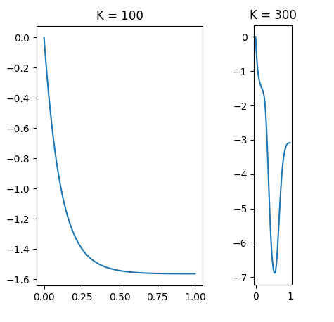
and I still get a solution for $K=500$,

$K=5000$ works too. It is also sufficient to simplify the initial guess to

x = logspace(-6,0,21); x[0]=0;
y = [0*x-pi/2, 0*x]

Related Solutions

Numerically solve this ODE: $y”’ \left(x\right)=-0.5\cdot y \left(x\right) \cdot y”\left( x \right) -0.05 $

Runge-Kutta can be used to solve systems of first-order ODE. Any high-order ODE can be rewritten as a system of first-order ODE's as is written in the article. The equation system written in article, together with the initial conditions for $y$, $f$ and $g$, can directly be plugged into any forwards-integrator, for example from Scipy, by providing it the right-hand-side of the first order ODE system. You will get an array of time-changing values of $y, f, g$ as an answer

Trying to solve a two-point boundary value problem on MATLAB

As you did, you first write the system as

$\begin{bmatrix} y_1' \\ y_2' \end{bmatrix} = \begin{bmatrix} y_2 \\ -(1+e^{y_1}) \end{bmatrix}, \; \; \; \; \begin{bmatrix} y_1(0) \\ y_2(0) \end{bmatrix} = \begin{bmatrix} 0 \\ u'(0) \end{bmatrix}$

in order to use a standard numerical method for ODEs.

So, the goal is to give the right value to $u'(0)$ in order to have $u(1)=1$. In your system, you have to guess the value of $y_2(0)$.

Of course you could do it by hand, but you can actually write a bisection method in order to find the correct value for the first derivative. The function you have to set to zero is, actually, $F=y_1(N)-1$.

So, assume to use a numerical method for solving your ODE, say explicit Euler (EE) (for sake of simplicity):

Consider two initial data $y_0= [0,a]^T$, $y_0=[0,b]^T$
Solve the ODE with (EE) those different initial values. Then you compute, for both the numerical solutions you get $f_a=y_1(N)-1$ and $f_b=y_1(N)-1$.
Compute the mean of $a,b$, call it $x_m$, and set another initial data $y_0=[0,x_m]^T$, and solve the ODE with (EE) and the last initial data and define $f_m=y_1(N)-1$.
Apply a standard bisection method: if $f_m \cdot f_a <0$, then $b=x_m$ and $f_b=f_m$, otherwise $a=x_m,f_a=f_m$
Repet the above procedure until the distance between $a$ and $b$ is $|b-a| \leq \epsilon$, where $\epsilon$ is a chosen tolerance

The following (runable) MatLab code computes the right value for $y_2(0)$, which is approximately $2.4592$.

fun=@(t,y) [y(2);-1-exp(y(1))];  
m=200; %time steps
tstar=1;
k=tstar/m;
t = linspace(0,tstar,m+1);
y=zeros(2,m+1);
a=-5;
b=5; % extreme initial points for bisection
iter=0;
maxit=100;
tol=1e-6; %tolerance

while (abs(b-a)>tol) && (iter<maxit)

y(:,1)=[0,a]; %a initial guess iniziale for y2

for n = 1:m
    y(:,n+1) = y(:,n)+k*fun(t(n),y(:,n)); %EE
end
fa=y(1,end)-1; %I have to set to zero F=y(1) - 1. (Want y(1)=1)

y(:,1)=[0,b];

for n = 1:m
    y(:,n+1) = y(:,n)+k*fun(t(n),y(:,n)); %EE
end
fb=y(1,end)-1;    


iter=iter+1;
xm=(a+b)/2;
y(:,1)=[0,xm];

for n = 1:m
    y(:,n+1) = y(:,n)+k*fun(t(n),y(:,n)); %EE
end

fm=y(1,end)-1;


if fa*fm<=0
    b=xm;
    fb=fm;
else 
    a=xm;
    fa=fm;
end

end


disp('The correct value is')
disp(xm)

%%%PLOT THE NUM SOLUTION%%

y=zeros(2,m+1);
y(:,1)=[0,2.4592];
for n = 1:m
     y(:,n+1) = y(:,n)+k*fun(t(n),y(:,n)); %EE
end
plot(t,y(1,:),'-*')

The correct numerical solution is the following