Please consider this problem and my solution to it. I get the feeling, my approach is way off.
Problem:
A normal population has a variance of $15$. If samples of size $5$ are
drawn from this population, what percentage an be expected to have
variances less than $10$.
Answer
The sample variance has a chi-square distribution with $4$ degrees of freedom. Also observe that $\frac{10}{15} = 0.666667$. That is, you need to adjust for the population variance. I then went to this website:
https://stattrek.com/online-calculator/chi-square.aspx
and I entered $4$ for the degrees of freedom and $0.666667$ for the Chi-Square
critical value. I then got an answer of $0.05$ but the book gets an answer of
$0.50$.
What did I do wrong?
Thanks,
Bob
Sampling Distribution of Variances
probabilitystatistics
Related Solutions
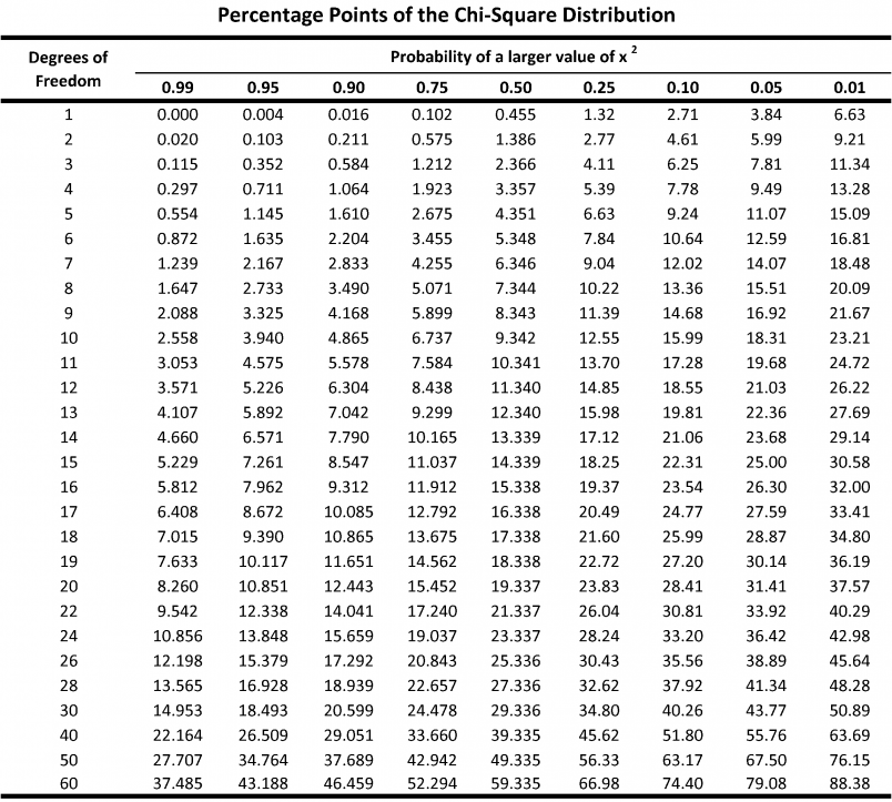
Most tables for the chi-square distribution are not designed to give you general probabilities; they are designed to give you critical values for specific tail probabilities corresponding to various significance levels. For example, refer to the following table:

To find $\Pr[X \le 6]$ using this table, you'd look up the sixth row, and try to find the column for which the entry in that table equals $6$. In other words, the sixth row and fifth column of this table means $\Pr[X > 5.348] \approx 0.5$, and the sixth row and seventh column means $\Pr[X > 7.84] \approx 0.25$. So in order to get $\Pr[X \le 6] = 1 - \Pr[X > 6]$, we would need a column somewhere in between $0.5$ and $0.25$, but it's not there in the table.
We can, however, use a crude linear interpolation: If we know that $\Pr[X > 5.348] = 0.5$ and $\Pr[X > 7.84] = 0.25$, then we can estimate that $$\Pr[X > 6] \approx 0.5 (1-\lambda) + 0.25 \lambda,$$ where $$ \lambda = \frac{6 - 5.348}{7.84 - 5.348} \approx 0.261637.$$ This gives $\Pr[X > 6] \approx 0.434591$, which gives $\Pr[X \le 6] \approx 0.565409$. It's not that bad an approximation; the actual answer calculated with a computer is $\Pr[X \le 6] = 0.57681\ldots$.
First, let's get the notation and definitions right; The sample mean $\bar X = \frac 1n\sum_{i=1}^n X_i.$ If the population mean $\mu$ is unknown and estimated by $\bar X,$ then the population variance $\sigma^2$ is estimated by the sample variance $S^2 = \frac{1}{n-1}\sum_{i=1}^n (X_i - \bar X)^2.$ Then $$\frac{(n-1)S^2}{\sigma^2} = \frac{\sum_{i-1}^n(X_i - \bar X)^2}{\sigma^2} \sim \mathsf{Chisq}(df = n-1).$$
For your dataset the statistics are:
x = c(22.2, 24.7, 20.9, 26.0, 27.0, 24.8, 26.5, 23.8, 25.6, 23.9)
n = length(x);  a = mean(x);  s = sd(x)
n;  a;  s
## 10           # sample size
## 24.54        # sample mean
## 1.912648     # sample SD
Then 95% confidence interval for the population variance $\sigma^2$ is obtained as $$((n-1)S^2/U,\, (n-1)S^2/L),$$ where $L$ and $U$ cut 2.5% of the probability from the lower and upper tails, respectively, of $\mathsf{Chisq(n-1)}.$ Computations of CIs for $\sigma^2$ and $\sigma$ in R statistical software follow:
UL = qchisq(c(.975, .025), n - 1);  UL
##  19.022768  2.700389
CI = (n-1)*s^2 / UL;  CI
##  1.730768 12.192315   95% CI for pop var
sqrt(CI)
##  1.315587 3.491750    95% CI for pop SD
Notice that $S = 1.913$ is contained in the CI for $\sigma$ as it must be, but that $S$ is not at the center of the CI, because the chi-squared distribution is skewed.
I assume you can use the appropriate quantiles of $\mathsf{Chisq}(9)$ to get 99% confidence intervals.
Addendum per Comments for 99% CIs: Of course, 99% confidence intervals have to be longer than 95% CIs.
 UL = qchisq(c(.995, .005), n - 1);  UL
 ##  23.589351  1.734933  # same as you showed in your question
 CI = (n-1)*s^2 / UL;  CI
 ##  1.395715 18.977103   # using correct numerator, this is different
 sqrt(CI)
 ## 1.181404 4.356272
Best Answer
Both look wrong to me. Your error is that the sample variance is proportional to a chi-square distribution with $4$ degrees of freedom, and you have missed this proportionality of $4$ or $5$ depending on how you calculate sample variances; you should try $4 \times \frac{10}{15}$ or $5 \times \frac{10}{15}$ rather than just $\frac{10}{15}$ as the value you are testing
If $X_1,X_2,\ldots,X_n$ were i.i.d. $\sim N(\mu,1)$, then I would have thought that $$\sum_i (X_i-\bar X)^2 = (n-1)\times \frac{1}{n-1}\sum_i (X_i-\bar X)^2 \sim \chi^2_{n-1}$$ so using R, I would have thought you would answer this question with
A simulation seems to produce a close figure:
But if the book's definition of sample variance is instead $\frac{1}{n}\sum_i (X_i-\bar X)^2$ rather than R's $\frac{1}{n-1}\sum_i (X_i-\bar X)^2$ then these would indeed become closer to $0.50$