In an idealized $n\times m$ room using $1\times 1$ tiles it would take $0$ cuts to lay tiles rectilinear pattern.
In an idealized $\sqrt2n \times \sqrt 2 m$ room, it will take $n+m$ cuts to lay tiles on the 45.
However rooms are never ideal. With the rectilinear pattern, it is only necessary to cut tiles along two walls
With the 45 pattern you must cut tiles along 4 walls.
When you can cut tiles exactly in half then you can tile that wall with fewer tiles as each diagonal is $\sqrt 2$ units long. But on the opposite wall, you need twice as many tiles, and Each tile piece is on average $\frac {\sqrt2}{2}$ units long.
Many of the trimmings are not reusable. Looking at your pattern when you cut with one big piece and one small piece, you keep using the big piece of one colored tile and the small piece of the other colored tile.
If the tiles are uniform in coloration, you can reuse more of your cuttings.
Putting this together, double looks to be more than just a rule of thumb. It would take some interesting coincidences to be too far off from that.
The problem in your code is
var nextVertex = intersectionPt
which should really be
var nextVertex = [0, 0]
(or at least a constant for all the tiles you generate).
The formula $\sum_{j=0}^4 n_j \mathbf e_j$ for the corner locations produces coordinates in a fixed coordinate system -- it's not relative to the intersection you start out with!
So the gaps you're seeing correspond to the distances between intersection points in the pentagrid, which you're erroneously adding to the tile coordinates.
A different problem that might bother you after you fix that is that the tiles you generate are too large compared to your pentagrid. You seem to be making the spacing between neighboring pentagrind lines equal to side length of the rhombs -- but the average distance between the "ribbons" corresponding to pentagrid lines is clearly longer than that. The tile side length is the width of a ribbon, and there's plenty of space left over between the ribbons!
(Image from https://www.ams.org/publicoutreach/feature-column/fcarc-ribbons)
This is not a problem for generating an infinite tiling, but it will make it difficult to predict which part of the pentagrid to look for intersections in, if you want to find all the tiles in a particular area of the coordinate system.
Curiously, none of your references seem to mention this difference in scale explicitly -- those that give actual formulas seem to assume that the lines on the pentagrid are unit spaced and that the rhomb sides are a unit apart. However, those references also don't actually show the complete pentagrid in the same plane as the finished Penrose tiling. Apparently in their view the pentagrid is only there to define which coordinate sets in $\mathbb Z^5$ correspond to corner points in the tiling, but the actual tiles live in a completely different coordinate system.
If you want each tile corner to appear roughly in the vicinity of the region of the pentagrid that corresponds to it, you need to scale one of the coordinate systems to match. Your sources don't give you the scaling factor to use, so let's derive it. We'll keep the tile side lengths as $1$, and figure out how far apart the pentagrid lines must be.
Suppose we're in the region of the pentagrid in your question with 5-coordinate tuple $(0,0,0,0,0)$, and we now move some large distance $D$ due right. What is the five-tuple corresponding to the region we land in, if the grid spacing is $G$?
Well, we move past $\frac DG$ red lines, crossing them at right angles. The orange lines make an angle of $72^\circ$ with the red ones, so the number of them we cross is an integer close to $\frac DG \cos 72^\circ$. The rounding becomes negligible when we let $D$ got to infinity, so just pretend it is $\frac DG\cos 72^\circ$ exactly. Similarly, the green lines make an angle of $144^\circ$ to the red ones, so the number of them we cross is $\frac DG \cos 144^\circ$. (The factor $\cos 144^\circ$ is negative, corresponding to the fact that we cross these lines in the direction of decreasing region coordinates). And so forth with the cyan and blue, with angles of $216^\circ$ and $288^\circ$.
All in all, we end up with the 5-coordinates, up to rounding
$$ (n_0,n_1,n_2,n_3,n_4) \approx \bigl(\tfrac DG,\tfrac DG\cos 72^\circ,\tfrac DG\cos 144^\circ,\tfrac DG\cos 216^\circ,\tfrac DG\cos 288^\circ\bigr). $$
The coordinates of the tile corner corresponding to that region is
$$ \sum_{j=0}^4 n_j \mathbf e_j = \sum_{j=0}^4 n_j \bigl(\cos(j\cdot 72^\circ), \sin(j\cdot 72^\circ)\bigr). $$
We're just interested in the $x$-coordinate, so plug in the $n_j$s above to get
$$ x \approx \frac DG \sum_{j=0}^4 \cos^2(j\cdot 72^\circ)
= \frac DG \sum_{j=0}^4 \frac{1 - \cos(j\cdot 144^\circ)}2
= \frac DG \cdot \frac{5-\sum_{j=0}^4 \cos(j\cdot 144^\circ)}2
= \frac DG \cdot \frac52 .
$$
(The last equals sign is because the sum of cosines is the change in $x$-coordinate from going all the way around a pentagram with unit sides).
If this $x$ is to grow at the same average rate as $D$, we must set
$$ G = \frac52. $$
Beware, however, that even if you scale the grid by this factor, you still won't get closer than the tiles being "roughly in the vicinity" of the grid intersections that represent them. The nice images in the presentations you link to make it look like each rhombus will contain the grid intersection it comes from -- but it's not possible to align the grid such that this is always the case, nor such that every tile corner is inside the grid region that you compute its location from.
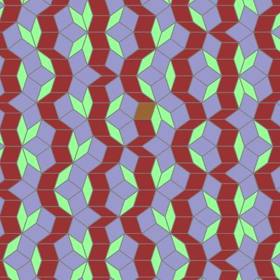
The pentagrid contains places where five grid lines almost but not quite meet in a point, like in this region of your pentagrid:

In this particular almost-intersection the fit is loose enough that we can see it's not exact -- but if your continue the pentagrid far enough, you will eventually find places where almost-intersections like this take place within arbitrarily small areas. The configuration has 6 internal regions and 10 actual intersections, and each of those intersections generates a full-sized tile in the final tiling. The 10 tiles come together in this pattern:

whose diameter is somewhat larger than the pentagrid spacing! Clearly not all of the tiles can lie directly above their defining intersection.
(We can see a differently oriented instance of this pattern in your buggy picture. Those tiles have particularly small gaps between them because the intersections that represent them are close together).
Best Answer
The set of tilings (which I'll call $T$) corresponds in number to the points on a line, so this essentially claims that $\lvert T\rvert=\lvert\mathbb R\rvert=\mathfrak c$. Instead of actually establishing a bijection, you can also establish two injections.
Upper bound on the cardinality
$\lvert T\rvert\le\lvert\mathbb R\rvert$ is easy: interpret $L,R,l,r$ as digits $0,1,2,3$ and the whole infinite sequence as a decimal fraction. Since the digit $9$ does not occur, you don't have to worry about things like $0.99\!\ldots=1$ so you know that every infinite sequence corresponds exactly to one real number. So you have an injective map from $T$ to $[0,1)\subset\mathbb R$.
Uncountability of sequences
$\lvert T\rvert\ge\lvert\mathbb R\rvert$ is harder. You could interpret rational numbers as fractions with base $4$, so every digit would correspond to one of the letters. You could also do the following preprocessing:
$$f(x):=\begin{cases} L,g(x) &\text{if } x\in[0,1) \\ R,g(1/x) &\text{if } x\in[1,\infty) \\ l,g(-x) &\text{if } x\in(-1,0) \\ r,g(-1/x)&\text{if } x\in(\infty,-1] \end{cases}$$
This will map any $x$ to the range $[0,1]$ which can then be used as input to the second function $g$ that represents that number in base $4$ and thus turns it into a sequence. You could write $1=0.333\!\ldots_4$ or tweak the definition of $f$ a bit (e.g. using $1-g(1/x)$ in the second case) to ensure that you only translate numbers from the range $[0,1)$ so that you can concentrate on the digits after the point.
Uncountability of point labels
So at this point, you have an injective function from $\mathbb R$ to infinite sequences in these four letters. But now you have a technical problem:
You have to work out the exact conditions of which sequences can and which can not be produced in this way. My guess is that you can show that there are only countably many forbidden sequences, so the remaining sequences would still be uncountably many.
Uncountability of tilings
As Daniel reminded me in a comment, what we have worked to so far (at least if you manage to show the countability of the sequences which are not tilings) demonstrates that there are uncountably many sequences describing a pattern seen from a given tile. But there are infinitely many tiles from which you could label the pattern and it would still be the same pattern that should be counted only once.
Two sequences denote the same pattern if they agree after some point $k$. So you can generate alternate labels for the same pattern by subsequently modifying elements of the sequence, starting at the first. You have four options for the first sequence item, and for each of them four for the second, and so on. You could explore all possible sequence modifications in a breadth first search, therefore there are only countably many (i.e. $\lvert\mathbb N\rvert=\aleph_0$) of these.
So why does that not break the uncountability of $T$? I'm not sure how you feel, but (at least at the moment) a counter-argument works best for me. Suppose there were only countably many tilings in $T$, represented by any suitable sequence for each. Then you could use the common $\mathbb N^2$ iteration: Take the original label of the first tiling, then the original label of the second tiling followed by the first modification of the first tiling, then the original label of the thirs tiling followed by the first modification of the second tiling followed by the second modification of the first tiling, and so on. In the end you'd enumerate all point labels, so there could only be $\lvert\mathbb N^2\rvert=\lvert\mathbb N\rvert=\aleph_0$ of these. This is a contradiction to the uncountability of label sequences we showed before.
Now that I think about it, this only shows $\lvert T\rvert>\aleph_0$ but one would need the continuum hypothesis to deduce $\lvert T\rvert=\mathfrak c$ from this. So if anyone has a better explanation (which still works on an intuitive level) of why $\mathfrak c/\aleph_0=\mathfrak c$ feel free to edit this post, comment, or provide your own answer.