So is the intuition correct that I shouldn't be concerned that the
overparameterized latent variables are not identifiable and aren't
fully converged when I take my posterior samples?
I think your intuition is correct: you shouldn't be concerned that the overparameterized latent variables are not identifiable and aren't
fully converged. In fact, the latent variables likely can't converge; my understanding is that in this situation the full state space chain is null recurrent, even though by your account there is a transformed state space of smaller dimension in which the chain is full recurrent (and hence has a stationary distribution). For what it's worth, I have deliberately created and used such MCMC chains myself in my applied research.
Sometimes stochastic processes with these features are used to model time series data (key word: cointegration). A quick look at this plot might generate some intuition:
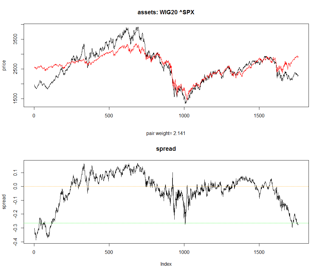
The upper figure shows two price time series, which one might think of as nonstationary in due to inflation even though no inflation can be seen on the time scale of the plot. Although each time series taken alone is nonstationary, there can exist a smaller dimensional manifold within the full state space (in this case, the "spread", i.e., the difference of the time series) such that the stochastic process generated by projecting the original process onto the manifold is stationary.
Are there some good references which discuss the use of non-identified latent variables in this way?
I don't know of any references that discuss the use of non-identified latent variables in this exact way, but here are a technical report and a published paper on the subject by Andrew Gelman, and here is a more recent manuscript by a different author that I think might be closer to what you're doing than the previous two references.
A recommendation: just compute the PSRF separately for each scalar component
The original article by Gelman & Rubin [1], as well as the Bayesian Data Analysis textbook of Gelman et al. [2], recommends calculating the potential scale reduction factor (PSRF) separately for each scalar parameter of interest. To deduce convergence, it is then required that all PSRFs are close to 1. It does not matter that your parameters are interpreted as random vectors, their components are scalars for which you can compute PSRFs.
Brooks & Gelman [3] have proposed a multivariate extension of the PSRF, which I review in the next section of this answer. However, to quote Gelman & Shirley [4]:
[...] these methods
may sometimes represent overkill: individual parameters can be well estimated even while
approximate convergence of simulations of a multivariate distribution can take a very long time.
Alternative: multivariate extension by Brooks&Gelman
Brooks & Gelman [3] propose a multivariate extension of the PSRF, where indeed one computes the estimated covariance matrix (your step 4) as a weighted sum of the within-chain ($W$) and between-chain ($B$) covariance matrices (your step 3):
\begin{equation}
\hat{V} = \frac{n-1}{n}W + \left ( 1 + \frac{1}{m} \right )\frac{B}{n},
\end{equation}
where $n$ is the chain length. Then, one needs to define some scalar metric for the distance between the covariance matrices $\hat{V},W$. The authors propose
\begin{equation}
\hat{R} = \max_a \frac{a^T\hat{V}a}{a^TWa} = \frac{n-1}{n} + \left(\frac{m+1}{m}\right)\lambda_1,
\end{equation}
where $m$ is the number of chains, the equality is shown in the article with $\lambda_1$ being the largest positive eigenvalue of $W^{-1}\hat{V}/n$. Then, the authors argue that under convergence of the chains, $\lambda_1\rightarrow 0$ and thus with big $n$ this multivariate $\hat{R}$ should converge near 1.
References
[1] Gelman, Andrew, and Donald B. Rubin. "Inference from iterative simulation using multiple sequences." Statistical Science (1992): 457-472.
[2] Gelman, Andrew, et al. Bayesian data analysis. CRC press, 2013.
[3] Brooks, Stephen P., and Andrew Gelman. "General methods for monitoring convergence of iterative simulations." Journal of Computational and Graphical Statistics 7.4 (1998): 434-455.
[4] Gelman, Andrew, and Kenneth Shirley. "Inference from simulations
and monitoring convergence". (Chapter 6 in Brooks, Steve, et al., eds. Handbook of Markov Chain Monte Carlo. CRC Press, 2011.)
All articles except the textbook [2] are available at Andrew Gelman's website Andrew Gelman's website.
Best Answer
Are you wondering how GR works, or why 1.1 seems to be the accepted cut-off. If the latter, you're not alone: arXiv paper questioning 1.1 cutoff argues that 1.1 is too high. They also propose a revised version of GR that is improved and can even evaluate a single chain.
The Stan folks are also working on a revised version of Stan's Rhat, which I believe is GR.
So if you're questioning 1.1, your instincts seem to be good. If you're questioning GR, the proposed revisions may also support your instincts.