I'm trying to understand my lecture notes but am a bit stuck on the concept of identifiability.
In one-way ANOVA, could someone please explain the reason for the constraint $\sum_{i=1}^{m} \beta_{j} = 0$ where we have m groups of observations, each group consisting of k observations with $Y_{ij}$ as the jth observation from the ith group, $E(Y_{ij}) = \mu + \beta_{i}, i = 1,…,m; j = 1,…,k, \text{Var}(Y_{ij}) = \sigma^{2}$and$ H_{0} : \beta_{1} = \beta_{2} = … = \beta_{m}$? I don't quite get the identifiability reason.
ANOVA – Understanding Sum-to-Zero Constraint in One-Way ANOVA and Identifiability Issues
anovageneralized linear modelidentifiability
Related Solutions
Both methods rely on the same idea, that of decomposing the observed variance into different parts or components. However, there are subtle differences in whether we consider items and/or raters as fixed or random effects. Apart from saying what part of the total variability is explained by the between factor (or how much the between variance departs from the residual variance), the F-test doesn't say much. At least this holds for a one-way ANOVA where we assume a fixed effect (and which corresponds to the ICC(1,1) described below). On the other hand, the ICC provides a bounded index when assessing rating reliability for several "exchangeable" raters, or homogeneity among analytical units.
We usually make the following distinction between the different kind of ICCs. This follows from the seminal work of Shrout and Fleiss (1979):
- One-way random effects model, ICC(1,1): each item is rated by different raters who are considered as sampled from a larger pool of potential raters, hence they are treated as random effects; the ICC is then interpreted as the % of total variance accounted for by subjects/items variance. This is called the consistency ICC.
- Two-way random effects model, ICC(2,1): both factors -- raters and items/subjects -- are viewed as random effects, and we have two variance components (or mean squares) in addition to the residual variance; we further assume that raters assess all items/subjects; the ICC gives in this case the % of variance attributable to raters + items/subjects.
- Two-way mixed model, ICC(3,1): contrary to the one-way approach, here raters are considered as fixed effects (no generalization beyond the sample at hand) but items/subjects are treated as random effects; the unit of analysis may be the individual or the average ratings.
This corresponds to cases 1 to 3 in their Table 1. An additional distinction can be made depending on whether we consider that observed ratings are the average of several ratings (they are called ICC(1,k), ICC(2,k), and ICC(3,k)) or not.
In sum, you have to choose the right model (one-way vs. two-way), and this is largely discussed in Shrout and Fleiss's paper. A one-way model tend to yield smaller values than the two-way model; likewise, a random-effects model generally yields lower values than a fixed-effects model. An ICC derived from a fixed-effects model is considered as a way to assess raters consistency (because we ignore rater variance), while for a random-effects model we talk of an estimate of raters agreement (whether raters are interchangeable or not). Only the two-way models incorporate the rater x subject interaction, which might be of interest when trying to unravel untypical rating patterns.
The following illustration is readily a copy/paste of the example from ICC() in the psych package (data come from Shrout and Fleiss, 1979). Data consists in 4 judges (J) asessing 6 subjects or targets (S) and are summarized below (I will assume that it is stored as an R matrix named sf)
   J1 J2 J3 J4
S1  9  2  5  8
S2  6  1  3  2
S3  8  4  6  8
S4  7  1  2  6
S5 10  5  6  9
S6  6  2  4  7
This example is interesting because it shows how the choice of the model might influence the results, therefore the interpretation of the reliability study. All 6 ICC models are as follows (this is Table 4 in Shrout and Fleiss's paper)
Intraclass correlation coefficients
                         type  ICC    F df1 df2       p lower bound upper bound
Single_raters_absolute   ICC1 0.17  1.8   5  18 0.16477      -0.133        0.72
Single_random_raters     ICC2 0.29 11.0   5  15 0.00013       0.019        0.76
Single_fixed_raters      ICC3 0.71 11.0   5  15 0.00013       0.342        0.95
Average_raters_absolute ICC1k 0.44  1.8   5  18 0.16477      -0.884        0.91
Average_random_raters   ICC2k 0.62 11.0   5  15 0.00013       0.071        0.93
Average_fixed_raters    ICC3k 0.91 11.0   5  15 0.00013       0.676        0.99
As can be seen, considering raters as fixed effects (hence not trying to generalize to a wider pool of raters) would yield a much higher value for the homogeneity of the measurement. (Similar results could be obtained with the irr package (icc()), although we must play with the different option for model type and unit of analysis.)
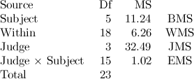
What do the ANOVA approach tell us? We need to fit two models to get the relevant mean squares:
- a one-way model that considers subject only; this allows to separate the targets being rated (between-group MS, BMS) and get an estimate of the within-error term (WMS)
- a two-way model that considers subject + rater + their interaction (when there's no replications, this last term will be confounded with the residuals); this allows to estimate the rater main effect (JMS) which can be accounted for if we want to use a random effects model (i.e., we'll add it to the total variability)
No need to look at the F-test, only MSs are of interest here.
library(reshape)
sf.df <- melt(sf, varnames=c("Subject", "Rater"))
anova(lm(value ~ Subject, sf.df))
anova(lm(value ~ Subject*Rater, sf.df))
Now, we can assemble the different pieces in an extended ANOVA Table which looks like the one shown below (this is Table 3 in Shrout and Fleiss's paper):

(source: mathurl.com)
where the first two rows come from the one-way model, whereas the next two ones come from the two-way ANOVA.
It is easy to check all formulae in Shrout and Fleiss's article, and we have everything we need to estimate the reliability for a single assessment. What about the reliability for the average of multiple assessments (which often is the quantity of interest in inter-rater studies)? Following Hays and Revicki (2005), it can be obtained from the above decomposition by just changing the total MS considered in the denominator, except for the two-way random-effects model for which we have to rewrite the ratio of MSs.
- In case of ICC(1,1)=(BMS-WMS)/(BMS+(k-1)•WMS), the overall reliability is computed as (BMS-WMS)/BMS=0.443.
- For the ICC(2,1)=(BMS-EMS)/(BMS+(k-1)•EMS+k•(JMS-EMS)/N), the overall reliability is (N•(BMS-EMS))/(N•BMS+JMS-EMS)=0.620.
- Finally, for the ICC(3,1)=(BMS-EMS)/(BMS+(k-1)•EMS), we have a reliability of (BMS-EMS)/BMS=0.909.
Again, we find that the overall reliability is higher when considering raters as fixed effects.
References
- Shrout, P.E. and Fleiss, J.L. (1979). Intraclass correlations: Uses in assessing rater reliability. Psychological Bulletin, 86, 420-3428.
- Hays, R.D. and Revicki, D. (2005). Reliability and validity (including responsiveness). In Fayers, P. and Hays, R.D. (eds.), Assessing Quality of Life in Clinical Trials, 2nd ed., pp. 25-39. Oxford University Press.
Your "assume also" clause equates two quadratic forms in $\mathbb{R}^n$ (with $\mathrm{y}=(y_1,y_2,\ldots,y_n)$ the variable). Since any quadratic form is completely determined by its values at $1+n+\binom{n+1}{2}$ distinct points, their agreement at all points of $\mathbb{R}^n$ is far more than needed to conclude the two forms are identical, whence their coefficients must be the same.
The coefficients of $y_1^2$ are $1/\sigma^2$ and $1/\nu^2$, whence $\sigma=\pm \nu$. We always stipulate that $\sigma$ and $\nu$ are nonnegative, implying $\sigma=\nu$. (The "real" parameter should be considered to be $\sigma^2$ or $1/\sigma^2$ rather than $\sigma$ itself.)
The linear terms in $y_i$ are both proportional to $b_0+b_1 x_i = a_0 + a_1 x_i$. Letting $\mathrm{1} = (1,1,\ldots, 1)$ and $\mathrm{x} = (x_1, x_2, \ldots, x_n)$, we conclude
$$(a_0 - b_0)\mathrm{1} + (a_1 - b_1)\mathrm{x} = \mathrm{0}.$$
Thus either
$\mathrm{1}$ and $\mathrm{x}$ are linearly independent, which by definition implies both $a_0 = b_0$ and $a_1 = b_1$, or
$\mathrm{1}$ and $\mathrm{x}$ are linearly dependent, which means $x_1 = x_2 = \cdots = x_n = x$, say. In that case
- If $x \ne 0$, $a_0 - b_0 = (a_1 - b_1) x$ determines one of $(a_0, a_1, b_0, b_1)$ in terms of the other three, or
- Otherwise $a_0=b_0$ and $a_1$ and $b_1$ could have any values.
In case (1) all parameters are uniquely determined: this is the identifiable model. In case (2) $\sigma = \nu$ is identifiable no matter what and various linear combinations of $(a_0,a_1,b_0,b_1)$ can be identified.
Evidently, linear independence of $\mathrm{x}$ and $\mathrm{1}$ is both necessary and sufficient for identifiability.
This criterion easily generalizes to multiple regression, where the ordinary least squares model is identifiable if and only if the design matrix $X$ (whose columns are formed from $\mathrm{1}, \mathrm{x}$, and any other variables in any order) has full rank: that is, there is no linear dependence among its columns.
Related Question
- Solved – If one of the samples has zero variance, can I perform an ANOVA or are pairwise one-sample t-test’s more appropriate
- Solved – One way unbalanced Anova and the sum to zero constraint
- Solved – Difference Between Full Model and Reduced Model in One-Way ANOVA
- ANOVA – Understanding Unusually High F Value in ANOVA
Best Answer
Consider for simplicity that $m=2$ and compare the models
$\mu=0,\beta_1=0,\beta_2=2$,
$\mu=1,\beta_1=-1,\beta_2=1$,
$\mu=2,\beta_1=-2,\beta_2=0$.
These models are all special cases of $(\mu,\beta_1,\beta_2)=(\mu,-\mu,2-\mu)$. You can see that whatever $\mu$ we choose, $\mu+\beta_1=0$ and $\mu+\beta_2=2$, so there's an infinite set of parameter-triples that match $E(Y_{1j})=0$ and $E(Y_{2j})=2$, and no way to distinguish between them.
Consequently, while data will allow you to estimate the two group-means, those two pieces of information (two df) - no matter how precisely estimated - are not going to be enough to estimate the three parameters (three df) in the model -- there's an extra degree of freedom that allows you to move all three parameters in particular ways relative to each other while keeping the group-means the same.
You need to restrict/constrain/regularize the situation in some way so that the model doesn't have more things to estimate than the design has the ability to identify.