The mean and variance of a Gaussian are the unknown parameters that specify that distribution in that case. Likewise, in topic modeling, you attempt to learn the unknown parameters of $K$ topics, where each topic is a multinomial distribution over words in the vocabulary. Thus, it is the parameters of each multinomial distribution (each topic) that you seek to infer.
Note that your learning algorithm will also output another set of multinomial paramaters that represent the distribution of topics for each document.
$\
\newcommand{\Mult}{\mathrm{Mult}}
\newcommand{\Dir}{\mathrm{Dir}}
\newcommand{\R}{\mathbb{R}}
$
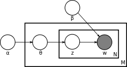
Let's briefly review the (unsmoothed) model of Latent Dirichlet Allocation, as presented in [Blei 2003].
[Blei 2003] Blei, David M., Andrew Y. Ng, and Michael I. Jordan. Latent dirichlet allocation. the Journal of machine Learning research 3 (2003): 993-1022.
For fixed vocabulary length $V$ and $K$ topics, $M$ documents, each with $N$ words,
$$
\begin{align}
\alpha &\in \R^K_+
& \text{Concentration Parameter} \\
\forall\, k \quad \beta_k &\in \R^{V}
& \text{Topic Probability Vectors} \\
\forall\, d \quad \theta_d | \alpha &\sim \Dir(\alpha)
& \text{Per-doc Topic Mixing Proportions} \\
\forall\, d,w \quad z_{dw} | \theta_d &\sim \Mult(\theta)
& \text{Per-word Topic Indicators} \\
\forall\, d,w \quad w_{dw} | \theta_d &\sim \beta_{z_{dw}}
& \text{Words (Observed)}
\end{align}
$$
Alternatively, $\beta=(\beta_1,\dots,\beta_K)$ and $\Theta=(\theta_1,\dots,\theta_M)$ can be represented as $K\times V$ and $D\times K$ probability matrices, respectively, where rows sum to one. $\mathbf{Z}=(z_{dj})_{d,j}$ and $\mathbf{W}=(w_{dj})_{d,j}$ can also be represented as matrices.
We model the documents themselves as mixtures of multinomial distributions. The mixing proportions $\theta_d$ for each document $d$ are conditionally independent of the mixing proportions for all other documents, given the concentration parameters $\alpha$. From [Blei 2003]:
The basic idea is that documents are represented as random mixtures over latent topics, where each topic is characterized as a distribution over words.
Typically, one observes the words $\mathbf{W}$ and is interested in inferring the values of the unknown variables $\Theta$, $\mathbf{Z}$ and $\beta$, and optionally the hyperparameters $\alpha$. In the paper, the inference procedure is presented as a Variational Expectation-Maximization algorithm, which essentially divides inference into two steps (c.f. Section 5.3), performed iteratively until convergence:
- (E-Step) Variational inference to (essentially) estimate the local hidden variables $\Theta$ and $\mathbf{Z}$ given estimates of $\alpha$ and $\beta$. This is done by optimizing over auxiliary variational parameters, whose expectation yields estimates of each hidden variable.
- (M-Step) Maximum likelihood estimation of global hidden variables $\alpha$ and $\beta$, given estimates of $\Theta$ and $\mathbf{Z}$.
The key here is that estimation on $\alpha$ is done as though we have complete information about the states of the local hidden variables. The hyperparameter $\alpha$ is the concentration parameter to a Dirichlet distribution, from which the multinomial probability vectors $\theta_d$ are "generated".
Crucially, the $\theta_d$ are all conditionally independent given $\alpha$, and $\alpha$ is conditionally independent of all other variables in the model given $\Theta$ (check the plate diagram!). Thus, estimation on $\alpha$ reduces to the problem of estimating the parameter of a Dirichlet distribution given a set of multinomial observations. The following papers derive algorithms to this end:
[Minka 2000] Minka, Thomas. Estimating a Dirichlet distribution. (2000): 3.
[Huang] Huang, Jonathan. Maximum likelihood estimation of Dirichlet distribution parameters.
For an example implementation of the $\alpha$-estimation procedure, you should check out gensim, which directly implements the Newton-Raphson update described in [Huang].
I would definitely recommend reading up about Expectation Maximization and Variational Inference if you aren't already familiar; intuition about these techniques is key to understanding what's happening in Blei's paper.
Best Answer
We see that pLSI describes a process for generating documents with topic distributions p(z | d) seen in a particular document in the collection as opposed to generating documents with arbitrary topic proportions from a prior probability distribution. This may not be crucial in information retrieval where the current document collection to be stored can be viewed as a fixed collection. However, in applications such as text categorization, it is crucial to have a model flexible enough to properly handle text that has not been seen before.
Thus probability of documents in pLSI are points (one point - one document from your collection), while in LDA, there is full topic simplex to use (of course, after training you have dirichlet distribution), so there are no problems to take new document.